The Terminology of Testing

Interact

We have just seen one example of a statistical hypothesis test. Using statistical tests as a way of making decisions is standard in many fields and has a standard terminology. Now it's time to formalize the sequence of the steps we take in most statistical tests.

Step 1: The Hypotheses¶

All statistical tests attempt to choose between two views of the world. These two views are called hypotheses. To choose between views, we use data. If our data are to be useful in distinguishing between two hypotheses, the hypotheses need to make different statements about how those data were generated.

The null hypothesis. This says that the data were generated at random under precisely-specified assumptions that can be simulated in a computer. The word "null" reinforces the idea that if the data look different from what the null hypothesis predicts, the difference is due to nothing but chance.

In the example about jury selection in Swain v. Alabama, the null hypothesis is that the panel was selected at random from the population of eligible jurors. This null hypothesis implies that, though the racial composition of the panel was different from that of the population of eligible jurors, there was no reason for the difference other than chance variation. Knowing the racial composition of the eligible population, we can simulate the panels we would get by randomly sampling from that population. So this null hypothesis does make precise assumptions about the data.

The alternative hypothesis. This says that some reason other than chance made the data differ from what was predicted by the null hypothesis. Informally, the alternative hypothesis says that the observed difference is "real."

In our example about jury selection, the alternative hypothesis is that the panel was not selected at random from the population of eligible jurors. Something other than chance led to the differences between the racial composition of the panel and the racial composition of the population of eligible jurors.

Notice that the alternative hypothesis does not need to say precisely how the data were generated. We only need to simulate what would happen if the null hypothesis were true. It would be impossible to simulate all the possible ways in which jury selection could be biased.

Step 2: The Test Statistic¶

In order to decide between the two hypothesis, we must choose a function that can summarize an observed or simulated dataset. It takes a dataset as its input and returns Informally, we will decide to accept the null hypothesis if our summary of the observed data is numerically similar to many of the summaries of the simulated data.

This function is called the test statistic. A statistic is a function that takes a dataset as its argument and returns a number, and a test statistic is a statistic that is used to summarize data for hypothesis testing.

In the example about jury panels, the test statistic we used was the number of black people in a jury panel. We did not actually define a function, but we could have defined this one:

def swain_test_statistic(panel):
    """Given a table of people that includes a 'Race' column, returns
    the number of rows for people labeled 'black'.
    """
    return panel.where("Race", are.equal_to("black")).num_rows

Computing the test statistic on the observed data is often the first computational step in a statistical test. In our example, the observed value of the test statistic was 8.

Step 3: Simulating data and test statistics we might have seen if the null hypothesis were true¶

This step sets aside the observed value of the test statistic, and instead focuses on what the value of the statistic might be if the null hypothesis were true.

Under the null hypothesis, the sample could have come out differently due to chance. So the test statistic could have come out differently, too. This step consists of repeatedly simulating datasets we would have seen under the null hypothesis of randomness, and computing the test statistic on each of those simulated datasets.

This produces a list of test statistics, one for each simulation. Usually we summarize this list by its distribution. In our example, we visualized this distribution by a histogram. Since 26% of the eligible population were black, the mass in this histogram was centered around 26.

Step 4. The Conclusion of the Test¶

The choice between the null and alternative hypotheses depends on the comparison between the results of Steps 2 and 3: the observed value of the test statistic and its distribution as predicted by the null hypothesis. We check whether they are consistent with each other.

Does the observed test statistic look like the test statistics we saw when we simulated under the null hypothesis? If so, the test does not point towards the alternative hypothesis; the null hypothesis is better supported by the data.

In our example about Swain's jury panel, the histogram of test statistics simulated under the null hypothesis was far away from the actual test statistic of 8.

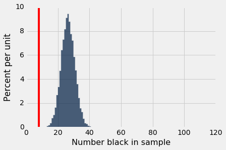
Histogram of null test statistics and observed test statistic

In cases like this, the data do not support the null hypothesis. That is why we concluded that the jury panel was not selected at random. Something other than random choice from the eligible population affected their composition.

If the data do not support the null hypothesis, we say that the test rejects the null hypothesis. In Swain's case, we rejected the null hypothesis.

The Terminology of Testing